Empirical Mean Estimates

Empirical mean estimates for distributions with same mean and variance but different kurtosis.

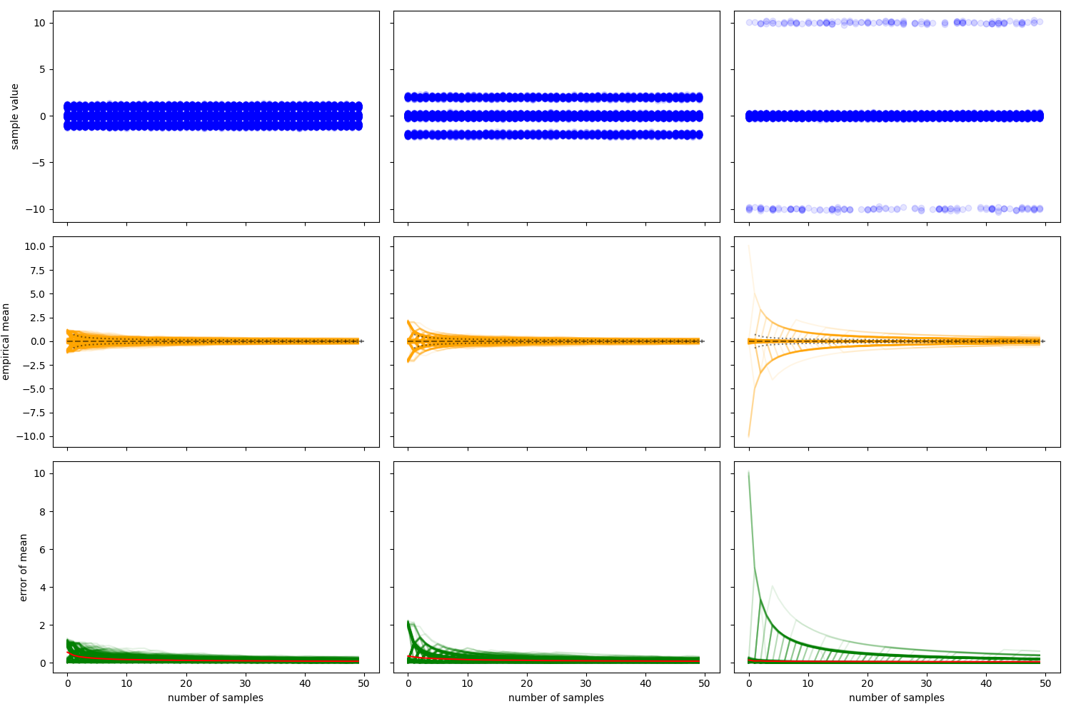
global_mean 0.0
global_var 0.51
global_std 0.714142842854285

global_mean 0.0
global_var 0.51
global_std 0.714142842854285

global_mean 0.0
global_var 0.51
global_std 0.714142842854285

import numpy as np
import matplotlib.pyplot as plt


# Define the parameters for the two Gaussian distributions
def define_mixture(means, stds, weights):
    means = np.asarray(means, float)
    stds = np.asarray(stds, float)
    weights = np.asarray(weights, float)
    if means.shape != stds.shape != weights.shape:
        raise ValueError("incompatible shapes")
    weights /= weights.sum()
    global_mean = (weights * means).sum()
    var_comp = (weights * stds ** 2).sum()
    mean_comp = (weights * (means - global_mean) ** 2).sum()
    global_var = var_comp + mean_comp
    global_std = np.sqrt(global_var)
    return means, stds, weights, global_mean, global_var, global_std

# Function to sample from the mixture distribution
def sample_from_mixture(n_samples, means, stds, weights):
    indices = np.random.choice(np.arange(len(means)), size=n_samples, p=weights)
    return np.random.normal(means[indices], stds[indices])

# define mixtures
mixture_std = 1e-1
mixtures = [
    define_mixture([-1, 0, 1], [mixture_std, mixture_std, mixture_std], [1, 2, 1]),
    define_mixture([-2, 0, 2], [mixture_std, mixture_std, mixture_std], [1, 14, 1]),
    define_mixture([-10, 0, 10], [mixture_std, mixture_std, mixture_std], [1, 398, 1]),
]

# Number of traces and number of samples per trace
n_trials = 1000
n_samples = 50

# plotting parameters
n_rows = 3
n_cols = len(mixtures)
x = np.arange(n_samples) + 1
fig, axs = plt.subplots(n_rows, n_cols, figsize=(15, 10), sharex='col', sharey='row')

for col_idx, (means, stds, weights, global_mean, global_var, global_std) in enumerate(mixtures):
    print(
        f"global_mean {global_mean}\n"
        f"global_var {global_var}\n"
        f"global_std {global_std}\n"
    )
    row_idx = -1

    # Initialize arrays to store samples and cumulative means
    all_samples = np.zeros((n_trials, n_samples))
    empirial_means = np.zeros((n_trials, n_samples))

    # Generate the samples and compute cumulative means
    for i in range(n_trials):
        samples = sample_from_mixture(n_samples=n_samples, means=means, stds=stds, weights=weights)
        all_samples[i] = samples
        empirial_means[i] = np.cumsum(samples) / np.arange(1, n_samples + 1)
    error_of_mean = np.abs(global_mean - empirial_means)
    average_error_of_mean = np.mean(error_of_mean, axis=0)

    # Plot the traces of the samples
    row_idx += 1
    ax = axs[row_idx, col_idx]
    for i in range(n_trials):
        ax.plot(all_samples[i], 'o', alpha=0.1, color='blue')
    if row_idx == n_rows - 1:
        ax.set_xlabel('number of samples')
    if col_idx == 0:
        ax.set_ylabel('sample value')

    # Plot the mean over time for each trace
    row_idx += 1
    ax = axs[row_idx, col_idx]
    for i in range(n_trials):
        ax.plot(empirial_means[i], alpha=0.1, color='orange')
    ax.plot([0, n_samples], [global_mean, global_mean], '--', color='black', alpha=0.5)
    ax.plot(x, global_mean + global_std / np.sqrt(x), ':', color='black', alpha=0.5)
    ax.plot(x, global_mean - global_std / np.sqrt(x), ':', color='black', alpha=0.5)
    if row_idx == n_rows - 1:
        ax.set_xlabel('number of samples')
    if col_idx == 0:
        ax.set_ylabel('empirical mean')

    # Compute and plot the average cumulative mean across all traces
    row_idx += 1
    ax = axs[row_idx, col_idx]
    for i in range(n_trials):
        ax.plot(error_of_mean[i], alpha=0.1, color='green')
    ax.plot(average_error_of_mean, color='red')
    if row_idx == n_rows - 1:
        ax.set_xlabel('number of samples')
    if col_idx == 0:
        ax.set_ylabel('error of mean')

fig.tight_layout()
plt.show()