Extract PCDs

Extract pitch-class distributions from a music file.

from pitchscapes.reader import sample_scape
from triangularmap import TMap

Get pitch-class scape with resolution n_time_intervals from MIDI or MXL

file_path = './JSB_Prelude_No_1_BWV_846_in_C_Major.mid'
scape = sample_scape(file_path=file_path, n_time_intervals=100, prior_counts=0, normalise=True)

Use TMap for slicing (need to reindex because of different ordering convention)

pcd_tmap = TMap(TMap.reindex_from_start_end_to_top_down(scape))

Extract NumPy array of dimension (n_time_intervals, 12) with PCDs from bottom level of pitch-class scape

pcds = pcd_tmap.lslice[1]
pcds.shape

(100, 12)

Some Plots

Getting key estimates / colours from PDC

import matplotlib.pyplot as plt
import numpy as np
from pitchscapes.plotting import key_scores_to_color
from pitchscapes.keyfinding import KeyEstimator

def key_colors(pcds: np.ndarray) -> np.ndarray:
    k = KeyEstimator()
    scores = k.get_score(pcds)
    colors = key_scores_to_color(scores, circle_of_fifths=True)
    colors = np.array([tuple(x) for x in colors])
    return colors

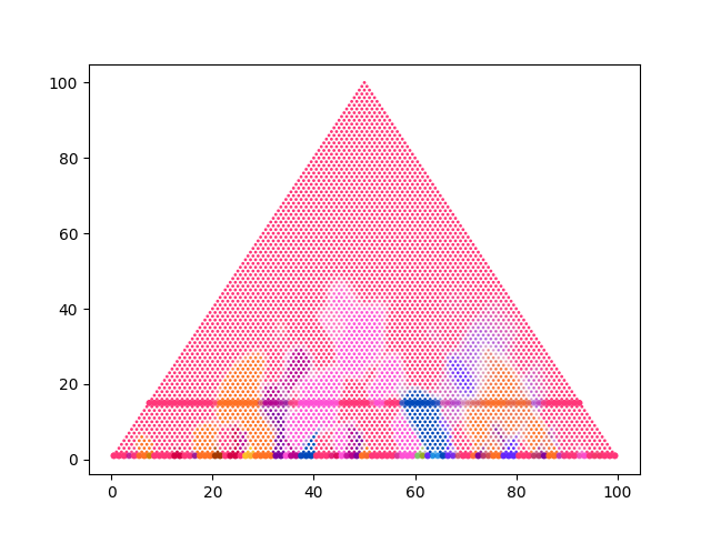
Doing key-scape plot as simple scatter plot

colours = key_colors(scape)
colour_tmap = TMap(TMap.reindex_from_start_end_to_top_down(colours))

# key-scape
x, y, c = [], [], []
for start in range(colour_tmap.n):
    for end in range(start + 1, colour_tmap.n + 1):
        x.append((start + end) / 2)
        y.append(end - start)
        c.append(colour_tmap[start, end])
plt.scatter(x=x, y=y, c=c, s=1)

# add single levels on top
x, y, c = [], [], []
for level in [1, 15]:
    for idx, col in enumerate(colour_tmap.lslice[level]):
        x.append(level / 2 + idx)
        y.append(level)
        c.append(col)
    plt.scatter(x=x, y=y, c=c, s=10)
plt.show()

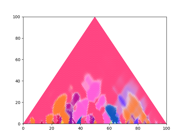
Do a proper key-scape plot from the colour array (start-end ordering)

from pitchscapes.plotting import scape_plot_from_array, key_legend

scape_plot_from_array(colours)
plt.show()

Same from the colour TMap (top-down ordering, so have to reindex back)

scape_plot_from_array(TMap.reindex_from_top_down_to_start_end(colour_tmap.arr))
plt.show()

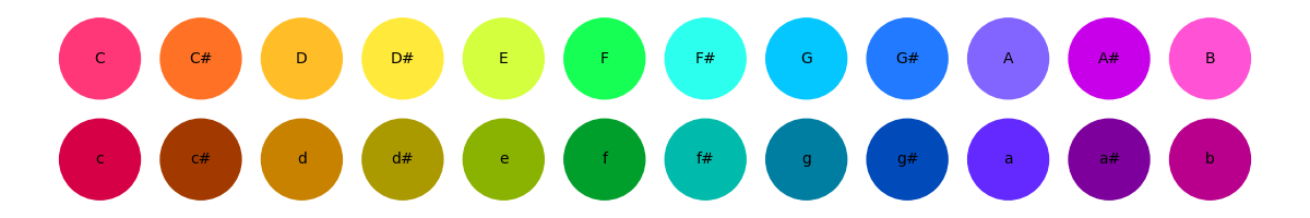
And plot a legend for reference

key_legend()
plt.show()

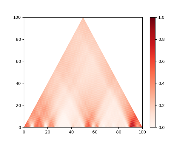
Plot a scalar value (here, value for first pitch)

import matplotlib as mpl

cmap = mpl.colormaps['Reds']
scape_plot_from_array(scape[:, 0], plot_kwargs=dict(vmin=0, vmax=1, cmap=cmap))
plt.colorbar(mpl.cm.ScalarMappable(cmap=cmap), ax=plt.gca())
plt.show()