Fourier Coefficients from PCDs

…

…

import numpy as np
import matplotlib.pyplot as plt


def dft(pcd, correct_mag=True):
    X = np.fft.rfft(pcd, norm="forward")
    # Compute magnitude and phase
    magnitude = np.abs(X)
    phase = np.angle(X)
    if correct_mag:
        magnitude *= 2
        magnitude[..., 0] /= 2
        magnitude[..., -1] /= 2
    return magnitude, phase


def continuous_reconstruction(t, mag, pha):
    x = 0
    for n, (m, p) in enumerate(zip(mag, pha)):
        x += m * np.cos(n * t + p * 2 * np.pi)
    return x
    # return (mag[None, :] * np.cos(np.arange(len(mag))[None, :] * (t[:, None] + pha[None, :] * 2 * np.pi))).sum(-1)


def show_coefficients(x, label):
    print("\n", label)

    # Compute the DFT
    mag, pha = dft(x)
    mag = mag.round(3)
    pha = (pha / (2 * np.pi)).round(3)

    # Print results
    # print("Fourier Coefficients (complex):", X)
    print("Magnitude:", mag)
    print("Phase (radians):", pha)

    plt.plot(np.arange(12), x)
    plt.plot(np.linspace(0, 11, 12),
             continuous_reconstruction(np.linspace(0, 2 * np.pi, 12, endpoint=False), mag, pha),
             '-o'
             )
    plt.show()

    print("\nn: mag | pha")
    for n, (m, p, label) in enumerate(zip(mag, pha, ["Zero", "One", "Two", "Three", "Four", "Five", "Six"])):
        # print(f"{n}: {m} | {p}")
        print(rf"\def\mag{label}{{{m}}}")
        print(rf"\def\phi{label}{{{p}}}")

    print("\nTable")
    print(r"coef. & mag. & phase \\")
    for n, (m, p, label) in enumerate(zip(mag, pha, ["Zero", "One", "Two", "Three", "Four", "Five", "Six"])):
        print(rf"\nth{{{n}}} & {m} & {p} \\")
    return plt.gcf()

fig = None
if __name__ == "__main__":
    # Albrecht C major
    x_chromatic = np.array([0.23800000000000004, 0.006000000000000002, 0.11100000000000003, 0.006000000000000002,
                            0.13700000000000004, 0.09400000000000003, 0.016000000000000004, 0.21400000000000005,
                            0.009000000000000001, 0.08000000000000002, 0.008000000000000002, 0.08100000000000002])

    # x_chromatic = np.array([1, 0, 0, 0,
    #                         0, 0, 0, 0,
    #                         0, 0, 0, 0])

    # x_chromatic = np.cos(6 * np.linspace(0, 2*np.pi, 12, endpoint=False) + 0*np.pi)
    fig = show_coefficients(x_chromatic, "chromatic")
fig

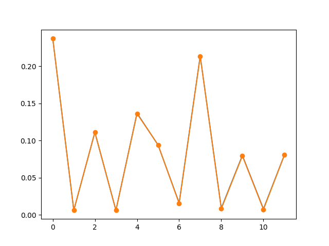
 chromatic
Magnitude: [0.083 0.006 0.039 0.046 0.01  0.091 0.003]
Phase (radians): [ 0.    -0.164 -0.012  0.072 -0.224  0.119  0.   ]

n: mag | pha
\def\magZero{0.083}
\def\phiZero{0.0}
\def\magOne{0.006}
\def\phiOne{-0.164}
\def\magTwo{0.039}
\def\phiTwo{-0.012}
\def\magThree{0.046}
\def\phiThree{0.072}
\def\magFour{0.01}
\def\phiFour{-0.224}
\def\magFive{0.091}
\def\phiFive{0.119}
\def\magSix{0.003}
\def\phiSix{0.0}

Table
coef. & mag. & phase \\
\nth{0} & 0.083 & 0.0 \\
\nth{1} & 0.006 & -0.164 \\
\nth{2} & 0.039 & -0.012 \\
\nth{3} & 0.046 & 0.072 \\
\nth{4} & 0.01 & -0.224 \\
\nth{5} & 0.091 & 0.119 \\
\nth{6} & 0.003 & 0.0 \\

<Figure size 640x480 with 1 Axes>

fig = None
if __name__ == "__main__":
    # chromatic profile
    x_CoF = x_chromatic[(np.arange(12) * 7) % 12]
    fig = show_coefficients(x_CoF, "circle of fifths")
fig

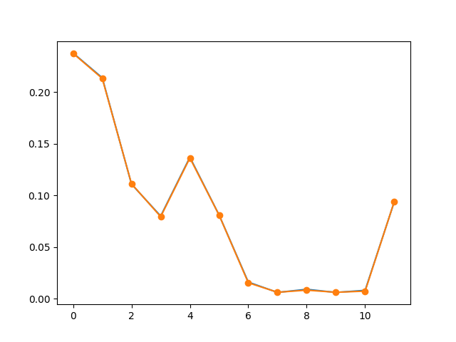
 circle of fifths
Magnitude: [0.083 0.091 0.039 0.046 0.01  0.006 0.003]
Phase (radians): [ 0.    -0.119 -0.012 -0.072 -0.224  0.164  0.   ]

n: mag | pha
\def\magZero{0.083}
\def\phiZero{0.0}
\def\magOne{0.091}
\def\phiOne{-0.119}
\def\magTwo{0.039}
\def\phiTwo{-0.012}
\def\magThree{0.046}
\def\phiThree{-0.072}
\def\magFour{0.01}
\def\phiFour{-0.224}
\def\magFive{0.006}
\def\phiFive{0.164}
\def\magSix{0.003}
\def\phiSix{0.0}

Table
coef. & mag. & phase \\
\nth{0} & 0.083 & 0.0 \\
\nth{1} & 0.091 & -0.119 \\
\nth{2} & 0.039 & -0.012 \\
\nth{3} & 0.046 & -0.072 \\
\nth{4} & 0.01 & -0.224 \\
\nth{5} & 0.006 & 0.164 \\
\nth{6} & 0.003 & 0.0 \\

<Figure size 640x480 with 1 Axes>