Optimising the Rosenbrock function

This runs stochastic gradient descent, specifically Adam, on the Rosenbrock function.

Define an Objective function module with loc and optimum that is later used for plotting.

from abc import ABC, abstractmethod

import torch
from torch.nn import Module, Parameter
from torch.optim import Adam
from torch.optim.lr_scheduler import LambdaLR


class Objective(Module, ABC):

    def __init__(self, loc, optimum):
        super().__init__()
        self.loc = Parameter(torch.Tensor(loc))
        self.optimum = torch.Tensor(optimum)

    @abstractmethod
    def loss(self, loc):
        raise NotImplementedError

    def forward(self):
        return self.loss(self.loc)

A simple quadratic objective (easy to solve)

class Quadratic(Objective):

    def __init__(self, loc, sigma=((1, 0), (0, 1)), optimum=(0, 0), div=1.):
        super().__init__(loc=loc, optimum=optimum)
        self.prec = torch.inverse(torch.Tensor(sigma))
        self.div = div

    def loss(self, loc):
        diff = loc - self.optimum
        return torch.einsum('...a,ab,...b->...', diff, self.prec, diff) / self.div

The Rosenbrock objective (hard to solve)

class RosenbrockFunction(Objective):
    def __init__(self, a=1.0, b=100.0, loc=(0, 0)):
        super().__init__(loc=loc, optimum=[a, a ** 2])
        self.a = a
        self.b = b

    def loss(self, loc):
        # Rosenbrock function calculation
        return (self.a - loc[..., 0]) ** 2 + self.b * (loc[..., 1] - loc[..., 0] ** 2) ** 2

A function for running the optimisation and plotting the results

import matplotlib.pyplot as plt

def optimise(module_kwargs,
             module_class=Quadratic,
             plot_range=((-10, 10), (-10, 10)),
             n_grid=50,
             n_iterations=100,
             lr=1.,
             warm_up=1
             ):
    # optimise and collect trace
    module = module_class(**module_kwargs)
    optimizer = Adam(module.parameters(), lr=lr)
    scheduler = LambdaLR(optimizer, lr_lambda=lambda step: step / warm_up if step < warm_up else 1)
    trace = [module.loc.clone().detach()]
    for it in range(n_iterations):
        optimizer.zero_grad()
        loss = module()
        loss.backward()
        optimizer.step()
        scheduler.step()
        trace += [module.loc.clone().detach()]

    # plot
    fig, ax = plt.subplots(1, 1, figsize=(10, 10))

    # plot objective landscape
    x_grid = torch.linspace(*plot_range[0], n_grid)
    y_grid = torch.linspace(*plot_range[1], n_grid)
    xy = torch.meshgrid([x_grid, y_grid])
    # flatten and concatenate along new dimension to get grid of coordinates
    locs = torch.cat(tuple(l.flatten()[..., None] for l in xy), dim=-1)
    # evaluate function on grid
    f = module.loss(locs).reshape(n_grid, n_grid).transpose(-2, -1)
    ax.contourf(x_grid, y_grid, f, 100, zorder=-10, cmap='Reds_r')

    # optimum
    ax.scatter(*module.optimum, marker='+', c='g', zorder=100, label='optimum')

    # trace
    c = (0.1, 0.1, 0.1)
    trace = torch.cat(tuple(t[None, :] for t in trace)).clone().detach().numpy()
    ax.plot(*trace.transpose(), '-o', linewidth=1, markersize=3, color=c, label='trace')
    ax.scatter(*trace[0], s=5, color=c, zorder=0)

    # adjust stuff
    ax.legend()
    ax.set_aspect('equal')
    ax.set_xlim(*plot_range[0])
    ax.set_ylim(*plot_range[1])

    fig.tight_layout()
    plt.show()

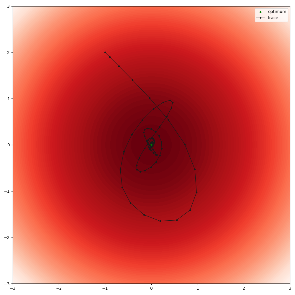
Run optimisation for simple quadratic objective (slightly too high learning rate to provoke overshooting)

optimise(
    module_class=Quadratic,
    module_kwargs=dict(loc=[-1, 2], sigma=[[1, 0], [0, 1]]),
    plot_range=((-3, 3), (-3, 3)),
    lr=1,
    warm_up=10,
)

/home/runner/.local/lib/python3.12/site-packages/torch/functional.py:554: UserWarning:

torch.meshgrid: in an upcoming release, it will be required to pass the indexing argument. (Triggered internally at /pytorch/aten/src/ATen/native/TensorShape.cpp:4322.)

For axis-aligned anisotropies, Adam’s adaptive learning rate works well

optimise(
    module_class=Quadratic,
    module_kwargs=dict(loc=[-2, 1], sigma=[[100, 0], [0, 1]]),
    plot_range=((-3, 3), (-3, 3)),
    lr=0.1,
    n_iterations=100,
    warm_up=10,
)

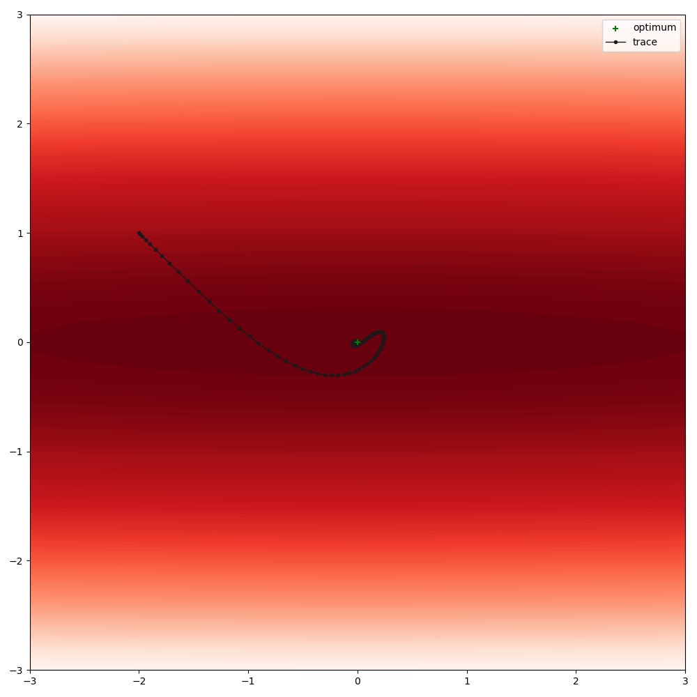
For non-aligned anisotropies, Adam’s adaptive learning rate fails (same settings)

optimise(
    module_class=Quadratic,
    module_kwargs=dict(loc=[-2, 1], sigma=[[1, -0.99], [-0.99, 1]]),
    plot_range=((-3, 3), (-3, 3)),
    lr=0.1,
    n_iterations=100,
    warm_up=10,
)

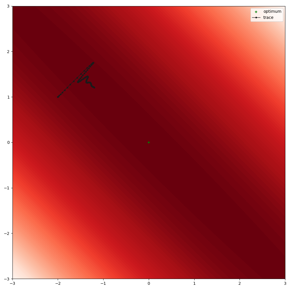
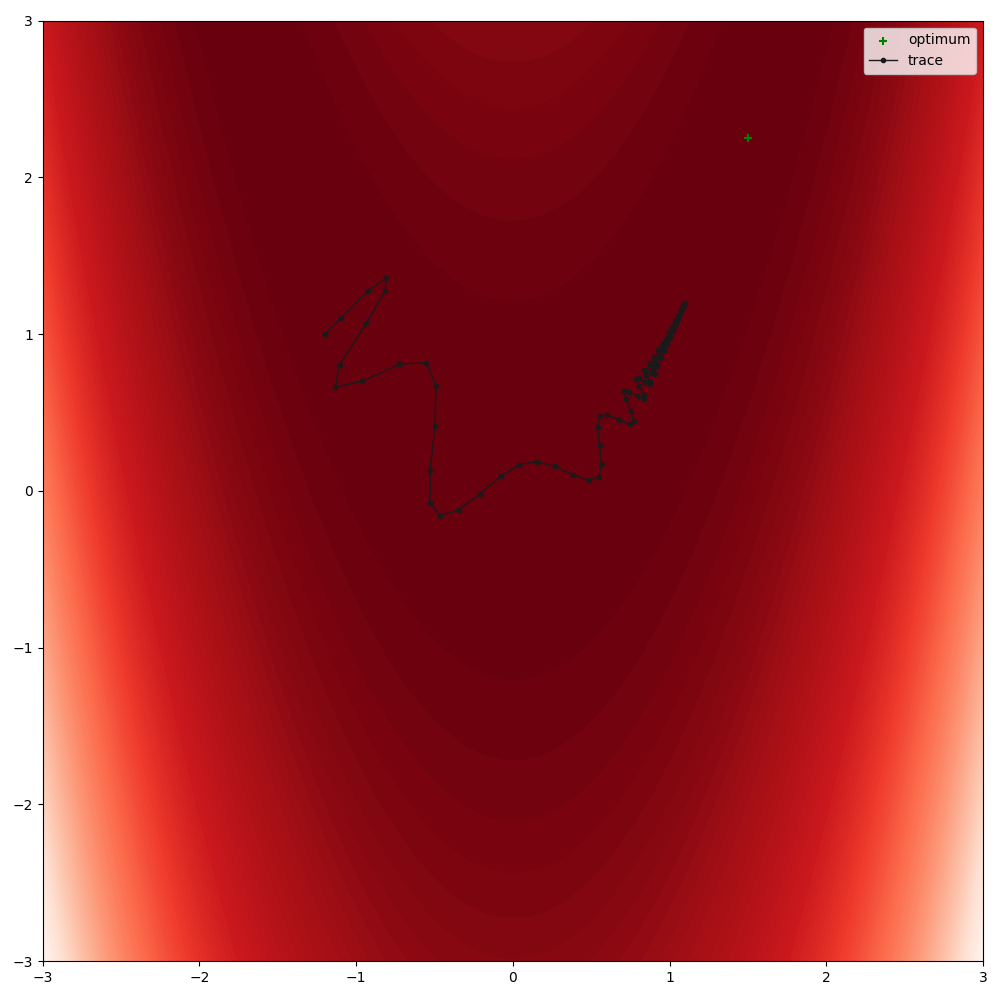
A non-trivial case where this becomes relevant is the Rosenbrock objective

optimise(
    module_class=RosenbrockFunction,
    module_kwargs=dict(a=1.5, b=100, loc=[-1.2, 1]),
    plot_range=((-3, 3), (-3, 3)),
    lr=1,
    warm_up=10,
)