Learning GP Kernel Combinations

import torch
import gpytorch
import matplotlib.pyplot as plt
torch.manual_seed(0)

<torch._C.Generator object at 0x7fb997745290>

Create toy data

GAP = True   # create a gap in the x data
STEP = True  # create a step in the y data

def y(x):
    y = torch.sin(2 * torch.pi * x * 5)
    if STEP:
        # optionally add a discontinuity
        y[x > 0.5] += 1
    return y

train_x = torch.linspace(0, 1, 100)
if GAP:
    train_x = train_x[(train_x < 0.2) + (train_x > 0.5)]
train_y = y(train_x) + 0.1 * torch.randn_like(train_x)

Build a weighted sum of standard kernels

# Each component gets its own ScaleKernel whose outputscale acts as the learnable weight.
def weighted_sum_kernel():
    k1 = gpytorch.kernels.ScaleKernel(gpytorch.kernels.RBFKernel())        # weight w1
    k2 = gpytorch.kernels.ScaleKernel(gpytorch.kernels.MaternKernel(nu=2.5))  # weight w2
    k3 = gpytorch.kernels.ScaleKernel(gpytorch.kernels.PeriodicKernel())   # weight w3
    # Sum defines a linear combination: w1*K1 + w2*K2 + w3*K3
    return k1 + k2 + k3

class ExactGP(gpytorch.models.ExactGP):
    def __init__(self, x, y, likelihood):
        super().__init__(x, y, likelihood)
        self.mean_module = gpytorch.means.ConstantMean()
        self.covar_module = weighted_sum_kernel()

    def forward(self, x):
        mean_x = self.mean_module(x)
        covar_x = self.covar_module(x)
        return gpytorch.distributions.MultivariateNormal(mean_x, covar_x)

likelihood = gpytorch.likelihoods.GaussianLikelihood()
model = ExactGP(train_x, train_y, likelihood)

Train hyperparameters and weights jointly with Adam

model.train()
likelihood.train()
optimizer = torch.optim.Adam(model.parameters(), lr=0.1)
mll = gpytorch.mlls.ExactMarginalLogLikelihood(likelihood, model)

for _ in range(300):
    optimizer.zero_grad()
    output = model(train_x)
    loss = -mll(output, train_y)
    loss.backward()
    optimizer.step()

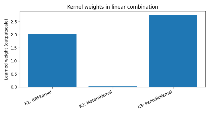
Inspect learned weights and internals

with torch.no_grad():
    # The sum kernel is a gpytorch.kernels.AdditiveKernel whose .kernels holds the components
    for i, sk in enumerate(model.covar_module.kernels, 1):
        w = sk.outputscale.item()                         # linear weight
        base = sk.base_kernel
        ls = base.lengthscale.detach().view(-1).tolist() if hasattr(base, "lengthscale") else None
        print(f"K{i}: {base.__class__.__name__}, weight={w:.3f}, lengthscale(s)={ls}")

K1: RBFKernel, weight=2.034, lengthscale(s)=[1.1811593770980835]
K2: MaternKernel, weight=0.017, lengthscale(s)=[1.5676146745681763]
K3: PeriodicKernel, weight=2.764, lengthscale(s)=[0.6790819764137268]

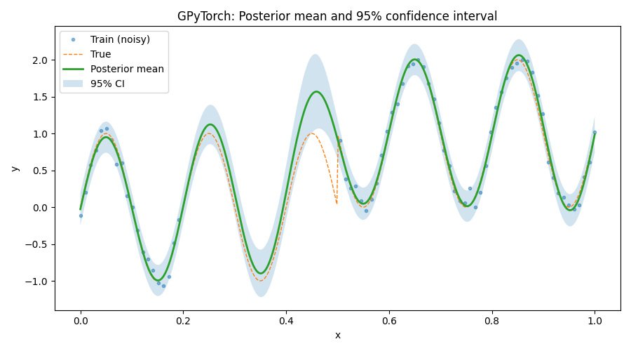
Plot results

# Switch to eval mode and make predictions on a dense grid
model.eval()
likelihood.eval()
test_x = torch.linspace(0, 1, 400)

with torch.no_grad(), gpytorch.settings.fast_pred_var():
    pred = likelihood(model(test_x))
    mean = pred.mean
    lower, upper = pred.confidence_region()

# Helper to move tensors to numpy
to_np = lambda t: t.detach().cpu().numpy()

Plot posterior with 95% confidence band

plt.figure(figsize=(9, 5))
plt.plot(to_np(train_x), to_np(train_y), ".", alpha=0.5, label="Train (noisy)")
plt.plot(to_np(test_x), to_np(y(test_x)), "--", lw=1, label="True")
plt.plot(to_np(test_x), to_np(mean), lw=2, label="Posterior mean")
plt.fill_between(to_np(test_x), to_np(lower), to_np(upper), alpha=0.2, label="95% CI")
plt.xlabel("x")
plt.ylabel("y")
plt.title("GPyTorch: Posterior mean and 95% confidence interval")
plt.legend(loc="best")
plt.tight_layout()
plt.show()

Bar chart of learned linear weights (ScaleKernel outputscales)

weights = []
names = []
for i, sk in enumerate(model.covar_module.kernels, 1):
    names.append(f"K{i}: {sk.base_kernel.__class__.__name__}")
    weights.append(sk.outputscale.item())

plt.figure(figsize=(7, 3.8))
plt.bar(names, weights)
plt.ylabel("Learned weight (outputscale)")
plt.title("Kernel weights in linear combination")
plt.xticks(rotation=25, ha="right")
plt.tight_layout()
plt.show()