Gaussian Process Outlier Detection

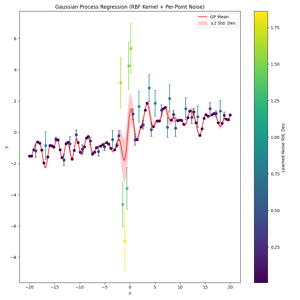
Using Gaussian Processes (GPs) to detect outliers/anomalies in data, with per-data-point noise variances. Plotting final results with color-coded error bars to indicate each point’s learned noise level.

import torch
import torch.optim as optim
import matplotlib.pyplot as plt
import matplotlib.cm as cm
import matplotlib.colors as mcolors

torch.manual_seed(0)

<torch._C.Generator object at 0x7fb997745290>

Create synthetic data with discontinuity

N = 100
min_data, max_data = -20, 20
x_train = torch.linspace(min_data, max_data, N).reshape(-1, 1)
f_true = 2 * torch.sigmoid(x_train) - 1
noise = 0.5 * torch.randn_like(f_true) / (f_true.abs() ** 5 + 1e-1)
y_train = f_true + noise

Setup GP

Define squared-exponential kernel

def rbf_kernel(X1, X2, lengthscale, variance):
    """
    k(x1, x2) = variance * exp(-(x1 - x2) ^ 2 / (2 * lengthscale ^ 2))
    """
    sqdist = (X1 - X2.T).pow(2)
    return variance * torch.exp(-0.5 * sqdist / lengthscale.pow(2))

Negative log marginal likelihood

def negative_log_marginal_likelihood(x, y, lengthscale, variance, noise_weights):
    """
    -log p(y|x) = 0.5*y^T(K^-1)*y + 0.5*log|K| + 0.5*N*log(2*pi),
    with K = RBF + diag(noise_weights).
    """
    K = rbf_kernel(x, x, lengthscale, variance)
    K = K + torch.diag(noise_weights)

    L = torch.linalg.cholesky(K)
    alpha = torch.cholesky_solve(y, L)
    log_det_K = 2.0 * torch.sum(torch.log(torch.diagonal(L)))

    N_data = x.shape[0]
    nll = 0.5 * y.T.mm(alpha) \
          + 0.5 * log_det_K \
          + 0.5 * N_data * torch.log(torch.tensor(2.0 * 3.141592653589793))
    return nll.squeeze()

Posterior prediction for new test points

def gp_posterior(x_train, y_train, x_test, lengthscale, variance, noise_weights):
    """
    Returns (mean, covariance) at x_test for GP with RBF kernel + per-data-point noise.
    """
    K_xx = rbf_kernel(x_train, x_train, lengthscale, variance)
    K_xx = K_xx + torch.diag(noise_weights)
    L = torch.linalg.cholesky(K_xx)

    K_xs = rbf_kernel(x_test, x_train, lengthscale, variance)
    K_ss = rbf_kernel(x_test, x_test, lengthscale, variance)

    alpha = torch.cholesky_solve(y_train, L)
    pred_mean = K_xs.mm(alpha)

    v = torch.linalg.solve(L, K_xs.T)
    pred_cov = K_ss - v.T.mm(v)

    return pred_mean, pred_cov

Train model

def train(
        n_steps=600,
        learn_weights=True
):
    lengthscale = torch.nn.Parameter(torch.tensor(1.0))
    variance = torch.nn.Parameter(torch.tensor(1.0))
    log_noise_weights = torch.nn.Parameter(torch.zeros(N) - 2.0)  # log-variance, init small

    params = [lengthscale, variance]
    if learn_weights:
        params.append(log_noise_weights)
    optimizer = optim.Adam(params, lr=0.03)

    nll_history = []

    for step in range(n_steps):
        optimizer.zero_grad()
        noise_weights = torch.exp(log_noise_weights)  # ensure positivity
        nll = negative_log_marginal_likelihood(
            x_train, y_train, lengthscale, variance, noise_weights
        )
        nll += noise_weights.sum()  # L1 penalty on noise weights
        nll.backward()
        optimizer.step()

        nll_history.append(nll.item())

        if (step + 1) % 50 == 0 or step == 0:
            print(
                f"Step {step + 1}/{n_steps}, NLL = {nll.item():.4f}, "
                f"lengthscale = {lengthscale.item():.4f}, "
                f"variance = {variance.item():.4f}, "
                f"noise (mean) = {noise_weights.mean().item():.4f}"
            )
    return nll_history, lengthscale, variance, log_noise_weights

Plot

def plot(nll_history, lengthscale, variance, log_noise_weights):

    # Plot final GP fit (mean + 2 std)
    # showing training points with error bars colored by noise level
    x_test = torch.linspace(min_data, max_data, 200).reshape(-1, 1)
    with torch.no_grad():
        noise_weights = torch.exp(log_noise_weights)
        pred_mean, pred_cov = gp_posterior(
            x_train, y_train, x_test, lengthscale, variance, noise_weights
        )
        pred_std = torch.sqrt(torch.diagonal(pred_cov))

    # Convert to numpy for plotting
    x_train_np = x_train.squeeze().numpy()
    y_train_np = y_train.squeeze().numpy()
    noise_std_np = torch.sqrt(noise_weights).detach().numpy()

    x_test_np = x_test.squeeze().numpy()
    pred_mean_np = pred_mean.squeeze().numpy()
    pred_std_np = pred_std.numpy()

    plt.figure(figsize=(10, 10))

    # Plot GP predictive mean +/- 2 std
    plt.plot(x_test_np, pred_mean_np, 'r', label='GP Mean')
    plt.fill_between(
        x_test_np,
        pred_mean_np - 2 * pred_std_np,
        pred_mean_np + 2 * pred_std_np,
        color='r', alpha=0.2, label='±2 Std. Dev.'
    )

    # Color-coded error bars for each training point
    norm = mcolors.Normalize(vmin=noise_std_np.min(), vmax=noise_std_np.max())
    cmap = cm.get_cmap('viridis')

    # Plot each data point with vertical error bars according to noise_std
    for i in range(len(x_train_np)):
        c = cmap(norm(noise_std_np[i]))
        plt.errorbar(
            x_train_np[i], y_train_np[i],
            yerr=noise_std_np[i],
            fmt='o', color=c, ecolor=c, capsize=3
        )

    # Add a colorbar to show how noise std maps to color
    sm = cm.ScalarMappable(norm=norm, cmap=cmap)
    sm.set_array([])  # needed in some older matplotlib versions
    cbar = plt.colorbar(sm, ax=plt.gca())
    cbar.set_label('Learned Noise Std. Dev.')

    plt.title('Gaussian Process Regression (RBF Kernel + Per-Point Noise)')
    plt.xlabel('x')
    plt.ylabel('y')
    plt.legend()
    plt.tight_layout()
    plt.show()

    # Plot training progress (NLL)
    plt.figure(figsize=(8, 4))
    plt.plot(nll_history, label='NLL')
    plt.xlabel('Iteration')
    plt.ylabel('Negative Log-Likelihood')
    plt.title('Training Progress')
    plt.legend()
    plt.tight_layout()
    plt.show()

    print("\nLearned parameters after training:")
    print(f"  lengthscale = {lengthscale.item():.4f}")
    print(f"  variance    = {variance.item():.4f}")
    print(f"  Mean noise weight = {noise_weights.mean().item():.4f}")

Run model

With learning weights

nll_history, lengthscale, variance, log_noise_weights = train(learn_weights=True)
plot(nll_history, lengthscale, variance, log_noise_weights)

• 
• 

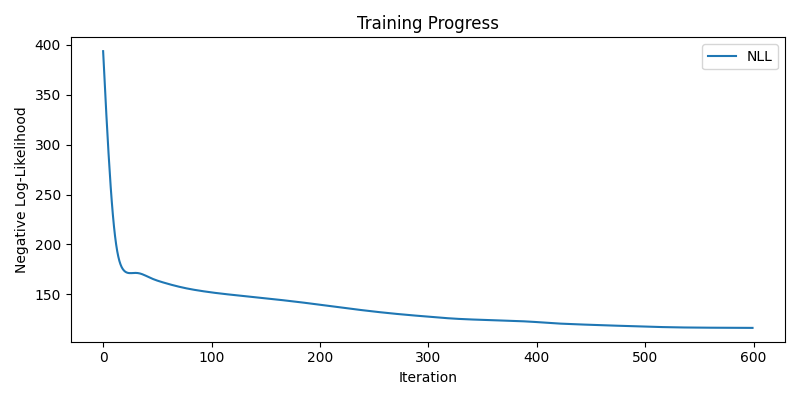
Step 1/600, NLL = 393.4452, lengthscale = 0.9700, variance = 1.0300, noise (mean) = 0.1353
Step 50/600, NLL = 164.2169, lengthscale = 0.4453, variance = 1.7800, noise (mean) = 0.0976
Step 100/600, NLL = 152.1879, lengthscale = 0.5481, variance = 1.9608, noise (mean) = 0.1114
Step 150/600, NLL = 146.2200, lengthscale = 0.5849, variance = 2.0953, noise (mean) = 0.1152
Step 200/600, NLL = 139.8615, lengthscale = 0.6172, variance = 2.1408, noise (mean) = 0.1182
Step 250/600, NLL = 133.0010, lengthscale = 0.6438, variance = 2.0798, noise (mean) = 0.1309
Step 300/600, NLL = 127.8574, lengthscale = 0.6669, variance = 1.8822, noise (mean) = 0.1552
Step 350/600, NLL = 124.5856, lengthscale = 0.6902, variance = 1.6446, noise (mean) = 0.1774
Step 400/600, NLL = 122.4225, lengthscale = 0.7060, variance = 1.4754, noise (mean) = 0.1884
Step 450/600, NLL = 119.6359, lengthscale = 0.7339, variance = 1.3657, noise (mean) = 0.2046
Step 500/600, NLL = 117.8596, lengthscale = 0.7424, variance = 1.1870, noise (mean) = 0.2219
Step 550/600, NLL = 116.8072, lengthscale = 0.7464, variance = 1.0759, noise (mean) = 0.2315
Step 600/600, NLL = 116.5449, lengthscale = 0.7481, variance = 1.0636, noise (mean) = 0.2325
/home/runner/work/snippets/snippets/examples/plot_gaussian_proces_outlier_detection.py:167: MatplotlibDeprecationWarning:

The get_cmap function was deprecated in Matplotlib 3.7 and will be removed in 3.11. Use ``matplotlib.colormaps[name]`` or ``matplotlib.colormaps.get_cmap()`` or ``pyplot.get_cmap()`` instead.


Learned parameters after training:
  lengthscale = 0.7481
  variance    = 1.0636
  Mean noise weight = 0.2325

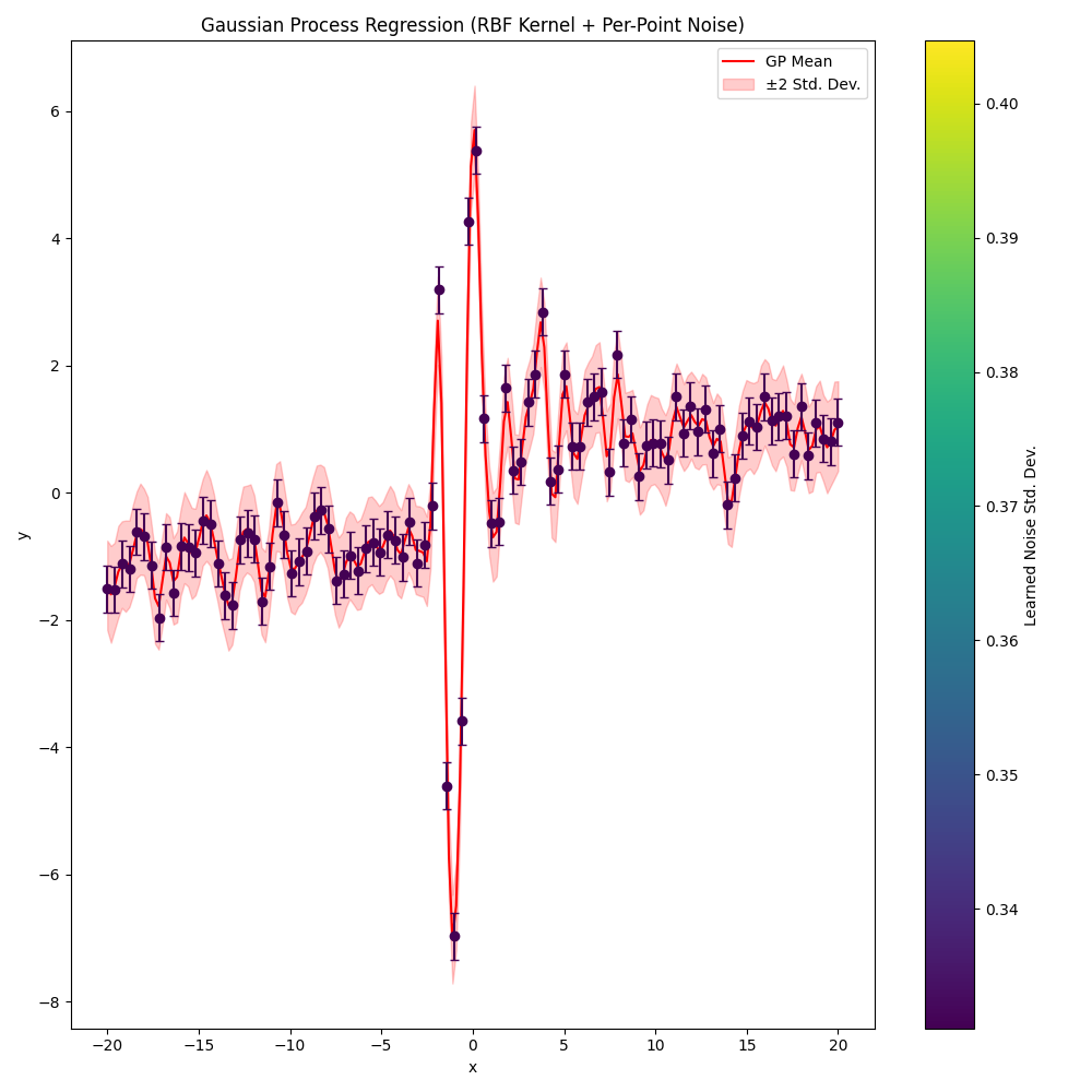
Without learning weights

nll_history, lengthscale, variance, log_noise_weights = train(learn_weights=False)
plot(nll_history, lengthscale, variance, log_noise_weights)

• 
• 

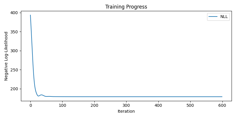
Step 1/600, NLL = 393.4452, lengthscale = 0.9700, variance = 1.0300, noise (mean) = 0.1353
Step 50/600, NLL = 179.6105, lengthscale = 0.3664, variance = 1.8482, noise (mean) = 0.1353
Step 100/600, NLL = 179.0276, lengthscale = 0.3769, variance = 2.0476, noise (mean) = 0.1353
Step 150/600, NLL = 178.8953, lengthscale = 0.3774, variance = 2.1564, noise (mean) = 0.1353
Step 200/600, NLL = 178.8651, lengthscale = 0.3791, variance = 2.2139, noise (mean) = 0.1353
Step 250/600, NLL = 178.8588, lengthscale = 0.3799, variance = 2.2421, noise (mean) = 0.1353
Step 300/600, NLL = 178.8577, lengthscale = 0.3802, variance = 2.2546, noise (mean) = 0.1353
Step 350/600, NLL = 178.8576, lengthscale = 0.3803, variance = 2.2595, noise (mean) = 0.1353
Step 400/600, NLL = 178.8575, lengthscale = 0.3804, variance = 2.2612, noise (mean) = 0.1353
Step 450/600, NLL = 178.8575, lengthscale = 0.3804, variance = 2.2617, noise (mean) = 0.1353
Step 500/600, NLL = 178.8575, lengthscale = 0.3804, variance = 2.2619, noise (mean) = 0.1353
Step 550/600, NLL = 178.8575, lengthscale = 0.3804, variance = 2.2619, noise (mean) = 0.1353
Step 600/600, NLL = 178.8575, lengthscale = 0.3804, variance = 2.2619, noise (mean) = 0.1353

Learned parameters after training:
  lengthscale = 0.3804
  variance    = 2.2619
  Mean noise weight = 0.1353